MapMind (Part II): Who Are Mindfulness Teachers?

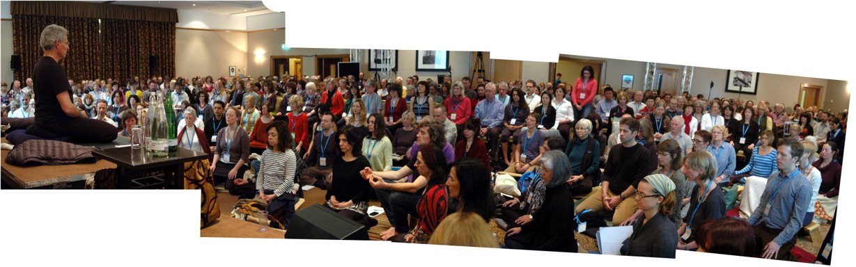
The project studied the people at the forefront of the mindfulness movement

1 Executive Summary

In Part II of the MapMind project, we ask “Who Are Mindfulness Teachers?”. We explore the demographics of mindfulness teachers. We use Exploratory Data Analysis (EDA) and data visualisation to reveal the hidden patterns in the survey data using descriptive statistics.

To understand the context of the attitudinal and behavioural data, we engage in an innovative synthesis of sense-making, data storytelling, and data visualisation.

Overall, we found mindfulness teachers tend to represent as majority:

• Female & Middle-Aged
• White, Heterosexual, Non-Disabled
• Highly Educated
• Work in High Status Occupations
• Middle-Class or White-Collar Professionals

“Mindfulness teachers” here refers to our sample of participants. But we need to be cautious about generalizing our findings to all mindfulness teachers. We return to this issue in the Discussion.

For an introduction to the overall project, including information about what data was collected, see MapMind (Part I).

2 Data Science Tools

We used the following data science libraries:

• Pandas:
  • A powerful Python data analysis toolkit.
  • Offers data structures like DataFrames and Series for handling and processing structured data.
  • Simplifies tasks such as data manipulation, cleaning, exploration, and visualization.
• Seaborn:
  • A Python visualization library based on Matplotlib.
  • Provides a high-level interface for drawing attractive and informative statistical graphics.
  • Ideal for exploring and understanding data through rich visualization capabilities.
• Matplotlib:
  • A comprehensive library for creating static, animated, and interactive visualizations in Python.
  • Offers extensive customization options for plots and charts.
  • Acts as a foundation for many other plotting libraries, including Seaborn.

Code

import requests
from io import BytesIO

import pandas as pd
import numpy as np
import matplotlib.pyplot as plt
import seaborn as sns

from sklearn.model_selection import train_test_split, cross_val_score, StratifiedKFold
from sklearn.ensemble import RandomForestClassifier
from sklearn.metrics import confusion_matrix, accuracy_score, cohen_kappa_score, roc_auc_score, classification_report
from sklearn.preprocessing import OneHotEncoder, StandardScaler
from sklearn.compose import ColumnTransformer
from sklearn.pipeline import Pipeline
from sklearn.model_selection import train_test_split
from xgboost import XGBClassifier

from scipy.stats import chi2_contingency

# Import the data from the SPSS file
survey = pd.read_spss("data/mm_survey_recoded-all-main_SPSS.sav")

Code

import pandas as pd

# Load the data
survey = pd.read_spss("data/mm_survey_recoded-all-main_SPSS.sav")

# Renaming columns (including the new columns from the R code)
survey.rename(columns={
    'Q5.2': 'motivations',
    'Q5.1': 'avenues_txt',
    'Q5.3': 'outlook',
    'Q5.4': 'outlook_txt',
    'Q6.1': 'age',
    'Q6.2': 'gender',
    'Q6.3': 'sexuality',
    'R6.4': 'ethnicity',
    'Q6.5': 'disability',
    'R2.25': 'technology',
    'Q7.2': 'website',
    'Q2.13': 'online_teaching',
    'Q2.14': 'online_n',
    'Q2.10': 'year_started',
    'R6.6': 'formal_education',
    'Q6.7': 'prof_qual',
    'R6.7_3': 'profession',
    'Q3.7': 'supervise_emp',
    'Q3.5': 'employment_other_type',
    'Q3.6': 'job_title',
    'Q2.23': 'trained',
    'Q2.24': 'trained_n',
    'R2.6_1': 'advocacy',
    'R2.6_2': 'business_entrepreneurial',
    'R2.6_3': 'management',
    'R2.11': 'courses_in_year',
    'Q2.12': 'clients_taught',
    'Q2.15': 'independent',
    'R2.16': 'nations',
    'R2.17': 'region_england',
    'R2.18': 'region_wales',
    'R2.19': 'region_scotland',
    'R.2.20': 'region_ireland',
    'R2.22': 'area',
    'R.2.21': 'contexts'
}, inplace=True)

category_columns = [
    'age', 
    'gender',
    'sexuality', 
    'ethnicity', 
    'disability', 
    'technology', 
    'website',
    'online_teaching', 
    'online_n', 
    'formal_education', 
    'prof_qual',
    'profession', 
    'supervise_emp', 
    'employment_other_type', 
    'trained',
    'trained_n', 
    'advocacy', 
    'business_entrepreneurial', 
    'management',
    'courses_in_year', 
    'clients_taught', 
    'independent', 
    'nations',
    'region_england', 
    'region_wales', 
    'region_scotland', 
    'region_ireland',
    'area', 
    'contexts',
]

for col in category_columns:
    if col in survey.columns:
        survey[col] = survey[col].astype('category')
    else:
        print(f"Column {col} not found in DataFrame.")

# Convert 'job_title' to string
survey['job_title'] = survey['job_title'].astype(str)

# Replace empty strings with NaN and convert to float
survey['year_started'] = survey['year_started'].replace('', np.nan).astype(float)

# Convert the entire series to nullable integer type Int64
survey['year_started'] = survey['year_started'].astype('Int64')

# Print some values of 'year_started' to check the transformation
#print(survey['year_started'].head())

# Save the modified DataFrame
survey.to_pickle('data/tidied_survey.pkl')

# Print number of users
#print(f"Total number of users after transform: {survey.shape[0]}")

3 Who are Mindfulness Teachers?

3.1 Majority Female & Middle-Aged

We asked our participants to report their gender and age.

We found mindfulness teachers in the U.K. tend to be female and middle-aged.

Code

import pandas as pd
import plotly.graph_objects as go

# Load the modified DataFrame
survey = pd.read_pickle('data/tidied_survey.pkl')

# Assuming 'survey.gender' contains the gender data
gender_data = survey['gender'].value_counts().reset_index()
gender_data.columns = ['Gender', 'Count']

# Creating a table with Plotly Graph Objects
fig = go.Figure(data=[go.Table(
    header=dict(values=list(gender_data.columns),
                fill_color='paleturquoise',
                align='left'),
    cells=dict(values=[gender_data.Gender, gender_data.Count],
               fill_color='lavender',
               align='left'))
])

fig.update_layout(title='Gender of Mindfulness Teachers')
fig.show()

# Function to create a bar chart remains the same
def create_bar_chart(data, var_name, flip_axes=False):
    # Filter out NA values
    filtered_data = data.dropna(subset=[var_name])

    # Create a bar chart using seaborn
    plt.figure(figsize=(10, 6))
    if not flip_axes:
        sns.countplot(x=var_name, data=filtered_data, palette="Set3", hue=var_name, legend=False)
        plt.xticks(rotation=45)  # Rotate x-axis labels if needed
    else:
        sns.countplot(y=var_name, data=filtered_data, palette="Set3", hue=var_name, legend=False)

    plt.title(f"Bar chart of {var_name}")
    plt.ylabel('Frequency' if not flip_axes else var_name)
    plt.xlabel(var_name if not flip_axes else 'Frequency')
    plt.show()

# Example usage of the function for 'age'
create_bar_chart(survey, 'age')

3.2 Majority White, Heterosexual, & Non-Disabled

We asked our participants to self-report their ethnicity, sexuality, and whether they considered themselves to have a disability.

We found they tended to self-report being white, heterosexual or straight, and non-disabled.

Code

import pandas as pd
import plotly.graph_objects as go
import plotly.express as px

# Load the modified DataFrame
survey = pd.read_pickle('data/tidied_survey.pkl')

# Convert data to long format for faceting
survey_long = survey.melt(id_vars=['ResponseId'], value_vars=['ethnicity', 'sexuality', 'disability'], var_name='demographic', value_name='value')

# Calculate frequency for each value within each demographic
survey_freq = survey_long.groupby(['demographic', 'value']).size().reset_index(name='freq')

# Remove NA values
survey_freq = survey_freq.dropna(subset=['value'])

# Rename "Non-white" to "People of colour" in ethnicity demographic
survey_freq.loc[(survey_freq['demographic'] == 'ethnicity') & (survey_freq['value'] == 'Non-white'), 'value'] = 'People of colour'

# Sort the frequencies in descending order
survey_freq.sort_values(by=['demographic', 'freq'], ascending=[True, False], inplace=True)

# Define the order of categories to be displayed
categories = ['ethnicity', 'sexuality', 'disability']
titles = ['Ethnicity of Mindfulness Teachers', 'Sexuality of Mindfulness Teachers', 'Disability Status of Mindfulness Teachers']

# Creating tables and plotting for each category in the defined order
for category, title in zip(categories, titles):
    # Filter data for the current category
    cat_data = survey_freq[survey_freq['demographic'] == category]

    # Creating a table with Plotly Graph Objects for the current category
    fig_table = go.Figure(data=[go.Table(
        header=dict(values=[category.capitalize(), 'Frequency'],
                    fill_color='paleturquoise',
                    align='left'),
        cells=dict(values=[cat_data['value'], cat_data['freq']],
                   fill_color='lavender',
                   align='left'))
    ])
    fig_table.update_layout(title=title)
    fig_table.show()

    # Creating a bar plot with Plotly Express for the current category
    fig_plot = px.bar(cat_data, x='freq', y='value', orientation='h', color='value', labels={'value': category.capitalize(), 'freq': 'Frequency'})
    fig_plot.update_layout(title=f'Distribution of {category.capitalize()}')
    fig_plot.show()

3.3 Majority Highly Educated

We asked our participants to report their highest level of formal education.

We found the majority of our sample self-reported as highly educated to higher degree level.

Code

import pandas as pd
import plotly.graph_objects as go

# Load the modified DataFrame
survey = pd.read_pickle('data/tidied_survey.pkl')

# Calculate frequencies in descending order
education_counts = survey['formal_education'].value_counts().sort_values(ascending=False)

# Calculate percentages
total_responses = survey['formal_education'].count()
education_percentages = (education_counts / total_responses) * 100

# Convert to DataFrame for Plotly
education_df = pd.DataFrame({
    'Formal Education': education_counts.index,
    'Frequency': education_counts.values,
    'Percentage': education_percentages.values
})

# Create table using Plotly Graph Objects
fig = go.Figure(data=[go.Table(
    header=dict(values=list(education_df.columns),
                fill_color='paleturquoise',
                align='left'),
    cells=dict(values=[education_df[k].round(2) if k == 'Percentage' else education_df[k] for k in education_df.columns], # Round percentages to 2 decimal places
               fill_color='lavender',
               align='left'))
])

fig.update_layout(title='Formal Education of Mindfulness Teachers')
fig.show()

# Create a countplot with bars in descending order of counts
plt.figure(figsize=(10, 6))
sns.set_style("whitegrid")
sns.countplot(data=survey, y='formal_education', hue='formal_education', palette='viridis', order=education_counts.index, legend=False)
plt.xlabel('Count')
plt.ylabel('Formal Education')
plt.title('Education Levels')
plt.show()

3.4 Majority Work in High Status Occupations

We asked participants to choose the type of their non-mindfulness employment from the following list:

1. Modern professional occupations (teacher, nurse, physiotherapist, social worker, welfare officer, artist, musician, police officer, software designer)
2. Traditional professional occupations (accountant, solicitor, medical practitioner, scientist, civil/mechanical engineer)
3. Senior managers or administrators (planning, organising and co-ordinating work, finance manager, chief executive)
4. Clerical and intermediate occupations (secretary, personal assistant, clerical worker, office clerk, call centre agent, nursing auxiliary, nursery nurse)
5. Middle or junior managers (office manager, retail manager, bank manager, restaurant manager, warehouse manager, publican)
6. Semi-routine manual and service occupations (postal worker, machine operative, security guard, caretaker, farm worker, catering assistant, receptionist, sales assistant)
7. Technical and craft occupations (motor mechanic, fitter, inspector, plumber, printer, tool maker, electrician, gardener, train driver)
8. Routine manual and service occupations (HGV driver, van driver, cleaner, porter, packer, sewing machinist, messenger, labourer, waiter/waitress, bar staff)

We found they tended to report working in high status employment types in their non-mindfulness work, with the majority working in modern professional occupations.

The analysis of the survey data reveals the following distribution of employment types among mindfulness teachers:

• The most common category is Modern professional occupations, with a frequency of 307, indicating a significant representation in this group.
• This is followed by Traditional professional occupations and Senior managers or administrators, with frequencies of 48 and 45, respectively.
• Less common categories include Clerical and intermediate occupations (14), Middle or junior managers (8), and both Semi-routine manual and service occupations and Technical and craft occupations with a frequency of 3 each. - The least common category is Routine manual and service occupations, noted only twice.

These results provide insights into the professional backgrounds of mindfulness teachers.

The following code loads the survey dataset, specifically focusing on the employment_other_type. It checks whether this variable is categorical and if it’s ordinal, then prints its categories. The code cleans the data by removing rows with NaN (‘Not a Number’) values and extracts the first part of the labels for conciseness. A visualization of the frequency of each employment type is generated, annotated with counts for clarity. The code maps these frequencies back to their original, longer labels, providing a comprehensive view of the employment types among mindfulness teachers.

Code

import pandas as pd
import matplotlib.pyplot as plt
import seaborn as sns

# Load the modified DataFrame
survey = pd.read_pickle('data/tidied_survey.pkl')

# Check if 'employment_other_type' is a categorical variable and if it is ordered
is_categorical = isinstance(survey['employment_other_type'].dtype, pd.CategoricalDtype)
is_ordered = survey['employment_other_type'].cat.ordered if is_categorical else False

# Remove rows where 'employment_other_type' is NaN
survey_clean = survey.dropna(subset=['employment_other_type']).copy()

# Extract the first part of the labels before the brackets
shortened_label_mapping = {label: label.split(' (')[0] for label in survey['employment_other_type'].cat.categories}
survey_clean['employment_other_type_short'] = survey_clean['employment_other_type'].map(shortened_label_mapping)

# Plot the frequencies of employment types with shortened labels
plt.figure(figsize=(10, 8))
employment_order_short = survey_clean['employment_other_type_short'].value_counts().index
ax = sns.countplot(y='employment_other_type_short', data=survey_clean, order=employment_order_short)
ax.set_title('Frequency of Employment Types')
ax.set_xlabel('Frequency')
ax.set_ylabel('Employment Type')

# Annotate the count on the bars
for p in ax.patches:
    ax.annotate(f'{int(p.get_width())}', (p.get_width(), p.get_y() + p.get_height() / 2), ha='left', va='center')

plt.tight_layout()
plt.show()

We studied the prevalent employment backgrounds among mindfulness teachers and their correlation with formal education levels, indicating a significant representation from professional and managerial fields. This shows that participants’ highest formal education is most commonly higher degree and their most common employment type is modern professional occupations.

The following code explores the relationship between employment types and formal education of mindfulness teachers. A PrettyTable and a bar plot display the count of formal education across various employment types, ordered by their frequency in the dataset.

Code

import pandas as pd
import matplotlib.pyplot as plt
import seaborn as sns
from prettytable import PrettyTable

import pandas as pd
import plotly.graph_objects as go

# Load the modified DataFrame
survey = pd.read_pickle('data/tidied_survey.pkl')

# Ensure 'employment_other_type' is treated as a categorical variable
survey['employment_other_type'] = pd.Categorical(
    survey['employment_other_type'],
    categories=survey['employment_other_type'].cat.categories,
    ordered=True
)

# Map employment types to numeric values (1-8) and create shortened labels
employment_mapping = {category: i for i, category in enumerate(survey['employment_other_type'].cat.categories, 1)}
reverse_mapping = {v: k for k, v in employment_mapping.items()}
shortened_label_mapping = {category: category.split(' (')[0] for category in survey['employment_other_type'].cat.categories}
survey['employment_type_numeric'] = survey['employment_other_type'].map(employment_mapping)
survey['employment_other_type_short'] = survey['employment_other_type'].map(shortened_label_mapping)

# Create a frequency table with numeric and shortened employment type labels
frequency_counts = survey['employment_type_numeric'].value_counts().reset_index()
frequency_counts.columns = ['Employment Type Numeric', 'Frequency']
frequency_table = frequency_counts.copy()
frequency_table['Employment Type'] = frequency_table['Employment Type Numeric'].map(lambda x: shortened_label_mapping[reverse_mapping[x]])

# Create a Plotly table
fig = go.Figure(data=[go.Table(
    header=dict(values=list(frequency_table.columns),
                fill_color='paleturquoise',
                align='left'),
    cells=dict(values=[frequency_table[k].tolist() for k in frequency_table.columns],
               fill_color='lavender',
               align='left'))
])

# Update the layout
fig.update_layout(
    title='Employment Types'
)

# Show the figure
fig.show()

# Determine the order of bars based on frequency count
numeric_order = [employment_mapping[cat] for cat in survey['employment_other_type'].value_counts().index]

# Create a plot showing the relationship between employment type and count of formal education
plt.figure(figsize=(12, 6))
sns.countplot(data=survey, x='employment_type_numeric', hue='formal_education', palette='viridis', order=numeric_order)
plt.xlabel('Employment Type (1-8)')
plt.ylabel('Count of Formal Education')
plt.title('Formal Education across Employment Types')
plt.xticks(ticks=range(len(numeric_order)), labels=[f'{i}' for i in numeric_order], rotation=45)
plt.legend(title='Formal Education')
plt.tight_layout()
plt.show()

3.5 Majority Middle-Class or White-Collar Professionals

Our data distribution suggests a diversity in the educational and professional backgrounds of mindfulness teachers, with a significant representation in middle and upper social classes. Our analysis of the survey data reveals the majority of teachers belong to the middle-white-collar_emp category (241 individuals), indicating a prevalent background in middle-class, white-collar professions. Upper-elite_emp is the next largest group (126 individuals), followed by working-blue-collar_emp (45 individuals), and upper-elite_plus (18 individuals).

To produce these results, we created a scoring system to classify the social class of mindfulness teachers, based on a combination of formal education, employment type, and roles in supervision or management. Teachers are categorized into Non-degree, Degree, and Higher degree for education, and their employment types are similarly classified. Additional points are awarded for supervisory and management roles, leading to four social class categories: working-blue-collar_emp, middle-white-collar_emp, upper-elite_emp, and ‘upper-elite_plus’.

The function calculate_social_class_score computes the social class score for mindfulness teachers based on their education (ed_class), employment type (emp_class), and roles in supervision and management. It uses a score_map where education and employment types are assigned scores: working-blue-collar and its employment counterpart are assigned 1 point, middle-white-collar and its employment equivalent get 2 points, and upper-elite categories receive 3 points.

The total base score for an individual is the sum of the points from their education and employment types. Additional bonus points are added based on their roles: 1 point if they have a supervisory role (supervise equals “Yes”) and 2 points for a management role (management equals “Yes”). The final score is a combination of the base score and any bonus points, reflecting their overall social class standing.

The following code analyzes the survey dataset and provides outsights into the distribution of social classes among survey respondents. The data is processed to classify individuals into different social classes based on their formal education, employment type, and work roles.

The following code processes the formal_education and employment_other_type columns to categorize them into different social classes. These categories are then used to calculate a social class score for each entry. The code also filters out irrelevant data (entries with Prefer not to say or missing employment types). After calculating the social class scores, the data is further classified into broader social class categories. The distribution of these classes is presented using a PrettyTable and a count plot. The table shows the frequency of each social class category, while the count plot visualizes the distribution of these categories in the dataset. This analysis and visualization help in understanding the composition of the dataset in terms of different social classes derived from education and employment types.

We discuss the potential limitations of our social class scoring system in the Conclusion.

Code

import pandas as pd

# Load the original DataFrame
survey = pd.read_pickle('data/tidied_survey.pkl')

# Create a new ordered categorical variable for 'formal_education'
education_order = ["Non-degree", "Degree", "Higher degree"]
survey['formal_education_ordered'] = pd.Categorical(survey['formal_education'], categories=education_order, ordered=True)

# Create a new variable based on 'formal_education_ordered'
def classify_education(edu):
    if edu == "Higher degree":
        return "upper-elite"
    elif edu == "Degree":
        return "middle-white-collar"
    elif edu == "Non-degree":
        return "working-blue-collar"
    else:
        return "unclassified"

survey['social_class_ed'] = survey['formal_education_ordered'].apply(classify_education)
survey['social_class_ed'] = pd.Categorical(survey['social_class_ed'], categories=["unclassified", "working-blue-collar", "middle-white-collar", "upper-elite"], ordered=True)

# Create a new variable 'employment_other_type_filtered' that filters out certain entries
survey['employment_other_type_filtered'] = survey['employment_other_type']
survey = survey[survey['employment_other_type_filtered'].notna() & (survey['employment_other_type_filtered'] != "Prefer not to say")]

# Apply transformation to 'employment_other_type_filtered'
def classify_employment(emp_type):
    # Replace with actual condition
    if "some condition or keyword for upper-elite_emp" in emp_type:
        return "upper-elite_emp"
    elif "some condition or keyword for middle-white-collar_emp" in emp_type:
        return "middle-white-collar_emp"
    elif "some condition or keyword for working-blue-collar_emp" in emp_type:
        return "working-blue-collar_emp"
    else:
        return "unclassified"

survey['social_class_emp'] = survey['employment_other_type_filtered'].apply(classify_employment)
survey['social_class_emp'] = pd.Categorical(survey['social_class_emp'], categories=["unclassified", "working-blue-collar_emp", "middle-white-collar_emp", "upper-elite_emp"], ordered=True)

# Calculate social class scores and create new variable
def calculate_social_class_score(ed_class, emp_class, supervise, management):
    score_map = {'working-blue-collar': 1, 'middle-white-collar': 2, 'upper-elite': 3,
                 'working-blue-collar_emp': 1, 'middle-white-collar_emp': 2, 'upper-elite_emp': 3}
    base_score = score_map.get(ed_class, 0) + score_map.get(emp_class, 0)
    bonus_points = 0
    if supervise == "Yes":
        bonus_points += 1
    if management == "Yes":
        bonus_points += 2
    return base_score + bonus_points

survey['social_scores'] = survey.apply(lambda row: calculate_social_class_score(
    row['social_class_ed'], row['social_class_emp'], row.get('supervise_emp', 'No'), row.get('management', 'No')), axis=1)

# Classify social class based on scores and create new variable
score_labels = ["working-blue-collar_emp", "middle-white-collar_emp", "upper-elite_emp", "upper-elite_plus"]
survey['social_class'] = pd.cut(survey['social_scores'], bins=[-float('inf'), 2, 4, 6, float('inf')], labels=score_labels, right=False)
survey['social_class'] = pd.Categorical(survey['social_class'], categories=score_labels)

# Continue with further analysis or save the DataFrame
survey.to_pickle('data/survey_social_class.pkl')

Code

import pandas as pd

# Load the survey dataframe
survey_clean = pd.read_pickle('data/tidied_survey.pkl')

# Load the modified DataFrame
survey_social_class = pd.read_pickle('data/survey_social_class.pkl')

# Check the number of rows and columns in survey_clean before the merge
#print("Before Merge - survey_clean shape:", survey_clean.shape)

# Merge the dataframes based on 'ResponseId' using a left join
survey_social_class_merged = survey_clean.merge(survey_social_class[['ResponseId', 'social_class']], on='ResponseId', how='left')

# Check the number of rows and columns in survey_social_class_merged after the merge
#print("After Merge - survey_social_class_merged shape:", survey_social_class_merged.shape)

# Now survey_social_class_merged contains the 'social_class' variable from survey_social_class

# Continue with further analysis or save the DataFrame
survey_social_class_merged.to_pickle('data/survey_social_class_merged.pkl')

Code

# Load the survey dataframe
survey_social_class = pd.read_pickle('data/survey_social_class.pkl')

# Load the survey dataframe
survey_social_class_merged = pd.read_pickle('data/survey_social_class_merged.pkl')

# Sample the same row numbers from the 'social_class' variable in both dataframes
row_numbers_to_sample = [1, 3, 5, 7]  # Replace with the row numbers you want to sample

# Check if the row numbers exist in both dataframes before sampling
common_row_numbers = set(row_numbers_to_sample) & set(survey_social_class.index) & set(survey_social_class_merged.index)

# Create a new list of row numbers that exist in both dataframes
common_row_numbers = list(common_row_numbers)

# Sample the 'social_class' variable for the common row numbers
sampled_social_class_survey_social_class = survey_social_class.loc[common_row_numbers, 'social_class']
sampled_social_class_survey_social_class_merged = survey_social_class_merged.loc[common_row_numbers, 'social_class']

# Print the descriptive summaries of the sampled 'social_class' variable in both dataframes
#print("Descriptive Summary of 'social_class' in survey_social_class:")
#print(sampled_social_class_survey_social_class.describe())

#print("\nDescriptive Summary of 'social_class' in survey_social_class_merged:")
#print(sampled_social_class_survey_social_class_merged.describe())

Code

import pandas as pd
import plotly.express as px
import plotly.graph_objects as go

# Load the modified DataFrame
survey = pd.read_pickle('data/survey_social_class_merged.pkl')

# Calculate the frequency and percentage of each social class
value_counts = survey['social_class'].value_counts()
total = value_counts.sum()
percentages = (value_counts / total) * 100

# Create a DataFrame for the table
table_df = pd.DataFrame({
    "Social Class": value_counts.index,
    "Frequency": value_counts.values,
    "Percentage": percentages.values
})

# Create a Plotly table
fig = go.Figure(data=[go.Table(
    header=dict(values=list(table_df.columns),
                fill_color='paleturquoise',
                align='left'),
    cells=dict(values=[table_df[k].tolist() for k in table_df.columns],
               fill_color='lavender',
               align='left'))
])

# Update the layout
fig.update_layout(
    title='Social Class of Mindfulness Teachers'
)

# Show the figure
fig.show()

# Prepare the DataFrame for Plotly Express
social_class_counts = survey['social_class'].value_counts().reset_index()
social_class_counts.columns = ['Social Class', 'Frequency']

# Plot the distribution of 'social_class' using Plotly Express
fig = px.bar(social_class_counts, x='Social Class', y='Frequency',
             title="Distribution of Social Classes Based on Total Score")
fig.update_xaxes(title_text='Social Class')
fig.update_yaxes(title_text='Number of Respondents')
fig.show()

# Optionally, print a sample of social class scores
#print("Sample of social class scores:\n", survey['social_scores'].sample(5))

4 Conclusion

This section gives a brief summary of the report, impact, limitations, and potential future work.

4.1 Overview

By putting people at the heart of research on technology, we have revealed hidden patterns in the data, the human stories behind the visualisations, and produced valuable outsights which can inform how the world could change.

On the one hand, the majority of our participants are a somewhat privileged group: white, heterosexual or straight, non-disabled, highly educated, working in high status occupations, with high social class status.

On the other hand, they are predominantly female and middle-aged.

4.2 Limitations & Future Potential

Overall, we need to be careful when interpreting the findings of our survey, and keep the following limitations in mind when evaluating our findings:

• While likely representing the majority of mindfulness teachers who were active during 2017-2021, our study mostly took place before the COVID-19 pandemic, which might have led to significant changes in the mindfulness field.

• We used a convenience sample, with voluntary participation. This design is potentially subject to a self-selection bias, where those who responded might have different characteristics to those who did not reply. Our sample might not be representative of the wider U.K. population.

• We could have situated our survey sample in relation to the U.K. population as a whole by integrating census data. This could be especially interesting for the geographical mapping presented in MapMind (Part I).

• We could pay more in-depth attention the experiences of participants in the minority of our sample: people of colour, of diverse sexualities, with working class backgrounds. We could explore these participants’ experiences in greater depth.

• The social class scoring system is based on understandings of the social status and the social hierarchies of employment, education, supervision, and management from sociology. Obviously, this data needs to be treated with some caution, because unlike the other demographic variables, we have classified the social class of our participants, based on their self-reported status. Nevertheless, it is striking the degree to which a majority of our participants have high level formal education, combined with high status occupations.

The study’s limitations, primarily its reliance on self-reported data and the need for broader demographic representation, pave the way for future research to build upon these findings and explore other influential factors in mindfulness teaching.

By putting people at the heart of the data revolution, we can reveal previously hidden inter-sectional patterns, thus promoting decision-making for fairer, more equal and sustainable futures.

We can use the tools of free and open science - especially Python - to make the findings of quantitative research, data analysis, and data science broadly accessible to a wide audience.